Place points randomly or in a grid within locations

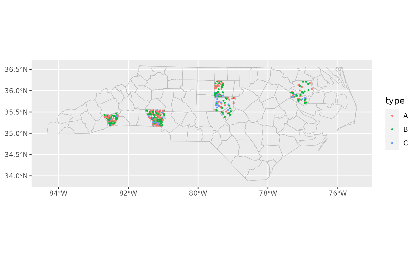
Each row of data is drawn as a single point inside the geographic area. This has similar strengths to a standard scatter plot, but has the potential to be misleading by implying that there is significance to the exact placement of the points.

Usage

geom_geoscatter(
  mapping = ggplot2::aes(),
  data = NULL,
  stat = "geoscatter",
  position = "identity",
  ...,
  feature_type = NA,
  sample_type = "random",
  inset = NA,
  map_base = "clip",
  map_inset = "auto",
  na.rm = TRUE,
  show.legend = "point",
  inherit.aes = TRUE
)

stat_geoscatter(
  mapping = NULL,
  data = NULL,
  geom = "sf_inset",
  position = "identity",
  ...,
  feature_type = NA,
  sample_type = "random",
  show.legend = NA,
  inherit.aes = TRUE
)

Arguments

mapping, data, stat, geom, position, na.rm, show.legend, inherit.aes, ...

See ggplot2::geom_sf().

feature_type

Type of map feature. See feature_types() for a list of registered types. If NA, the type is guessed based on the values in feature_names.

sample_type

sampling type (see the type argument of sf::st_sample()). "random" will place points randomly inside the boundaries, whereas "regular" and "hexagonal" will evenly space points, leaving a small margin close to the boundaries.

inset

Inset configuration; see configure_inset(). If NA (the default), this is inherited from the coord (see coord_sf_inset()).

map_base

Controls the layer with the base map. Possible values are "normal" to create a layer as though the inset were not specified, "clip" to create a layer with the inset viewport cut out, and "none" to prevent the insertion of a layer for the base map.

map_inset

Controls the layer with the inset map. Possible values are "auto" to choose the behaviour based on whether inset is specified, "normal" to create a layer with the viewport cut out and transformed, and "none" to prevent the insertion of a layer for the viewport map.

Value

A ggplot layer.

Aesthetics

The location aesthetic is required. geom_geoscatter() understands the same aesthetics as ggplot2::geom_point().

Computed variables

x

longitude

y

latitude

Examples

library(ggplot2)

cartographer::nc_type_example_2 |>
  ggplot(aes(location = county)) +
  geom_boundaries(feature_type = "sf.nc") +
  geom_geoscatter(aes(colour = type), size = 0.5) +
  coord_automap(feature_type = "sf.nc")