Use 'cartographer' to attach a spatial column to the data based
on place names in another column. The spatial data is then reduced to
coordinates in the same way as stat_sf_coordinates().
Usage
stat_automap_coords(
  mapping = NULL,
  data = NULL,
  geom = "sf_inset",
  position = "identity",
  ...,
  feature_type = NA,
  na.rm = TRUE,
  inset = waiver(),
  fun.geometry = NULL,
  show.legend = NA,
  inherit.aes = TRUE
)
Arguments
- mapping, data, geom, position, na.rm, show.legend, inherit.aes, fun.geometry, ...
- feature_type
Type of map feature. See
feature_types()for a list of registered types. IfNA, the type is guessed based on the values infeature_names.- inset
Inset configuration; see
configure_inset(). Ifwaiver(), the default, this is inherited from the coord (seecoord_sf_inset()).
Computed variables
- geometry
sfgeometry column representing the points- x
X dimension of the simple feature
- y
Y dimension of the simple feature
- x_inset
X dimension of the simple feature after inset transformation
- y_inset
Y dimension of the simple feature after inset transformation
- inside_inset
logical indicating points inside the inset viewport
- inset_scale
1 for points outside the inset, otherwise the configured inset scale parameter
Aesthetics
stat_automap_coords() understands the following aesthetics. Required aesthetics are displayed in bold and defaults are displayed for optional aesthetics:
| • | location | |
| • | group | → inferred |
| • | x | → after_stat(x) |
| • | y | → after_stat(y) |
Learn more about setting these aesthetics in vignette("ggplot2-specs").
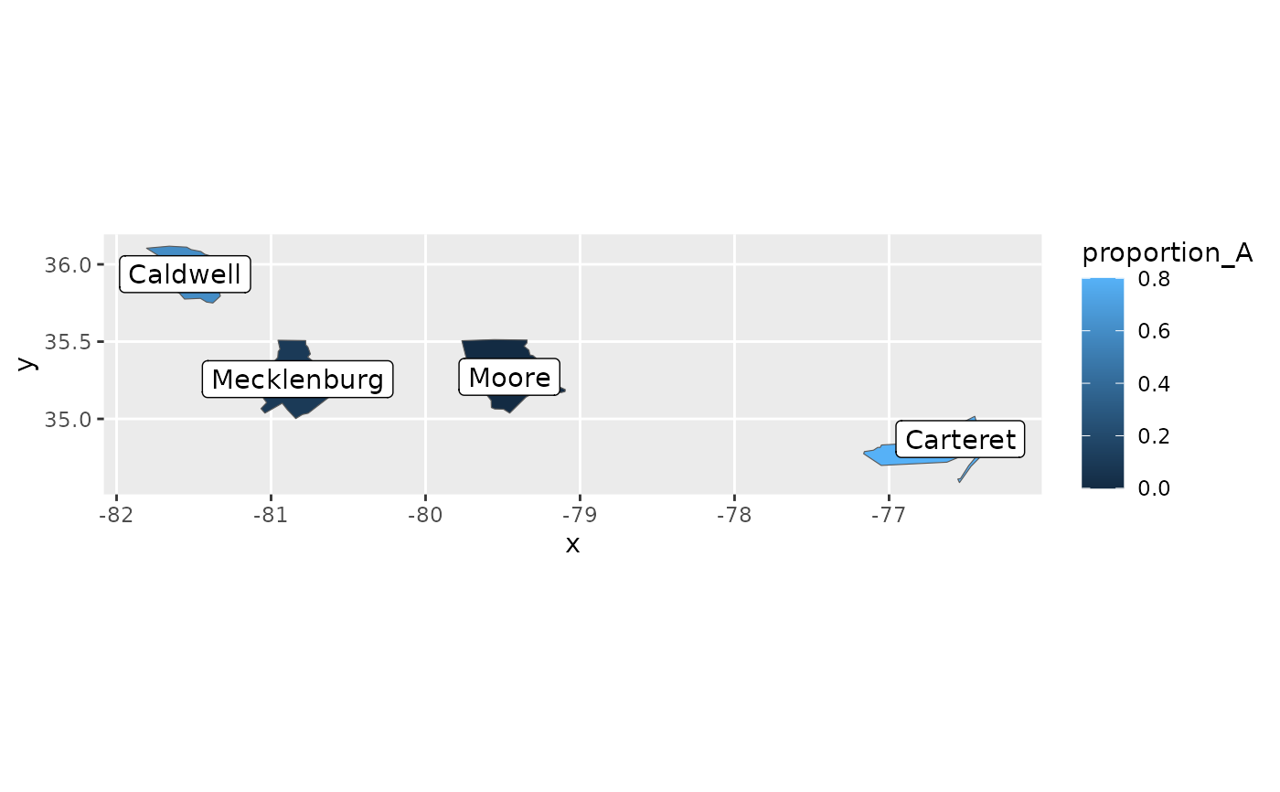
Examples
library(ggplot2)

events <- data.frame(
  county = c("Mecklenburg", "Carteret", "Moore", "Caldwell"),
  proportion_A = c(0.1, 0.8, 0.0, 0.6)
)

ggplot(events, aes(location = county)) +
  geom_sf(aes(fill = proportion_A), stat = "automap") +
  geom_label(aes(label = county), stat = "automap_coords") +
  coord_automap(feature_type = "sf.nc")